Applying CellPhenoX to Ulcerative Colitis Fibroblasts (single-cell transcriptomics)
Goal: Identify subtle, fibroblast-specific phenotypic changes associated with differing levels of inflammation
This tutorial explores the utility of CellPhenoX within a specific cell type. Using the single-cell transcriptomics data from Smillie et al., we (a) create the latent dimensions for the neighborhood abundance matrix (NAM), (b) train a random forest model to predict inflamed vs. non-inflamed status, and (c) visualize the resulting CellPhenoX Interpretable Score.
Importing Dependencies
[1]:
import pyCellPhenoX

import pandas as pd
/Users/zhanglab/Documents/Python Projects/pyCellPhenoX/pycpx/lib/python3.12/site-packages/tqdm/auto.py:21: TqdmWarning: IProgress not found. Please update jupyter and ipywidgets. See https://ipywidgets.readthedocs.io/en/stable/user_install.html
  from .autonotebook import tqdm as notebook_tqdm
Step 1: Import data
The expression file is expected to be a cells by gene matrix, and the meta file is expected to be a cells by meta data features matrix.
[3]:
# paths to expression data and meta data files
expression_file = "/example_UC_data/fibroblast_exp.csv"
meta_file = "/example_UC_data/fibroblast_met.csv"
output_path = "/output/"
# read in data
expression_mat = pd.read_csv(expression_file, index_col=0)
meta = pd.read_csv(meta_file, index_col=0)
[4]:
expression_mat.head()
[4]:
| ADAMDEC1 | ACTA2 | TAGLN | CCL11 | CCL13 | APOE | CXCL14 | CFD | CCL8 | CCL2 | ... | CCDC23 | MEIS1 | AP001258.4 | FBXO42 | ASUN | ELP6 | CCDC77 | ELK3 | INO80E | FHOD3 | |
|---|---|---|---|---|---|---|---|---|---|---|---|---|---|---|---|---|---|---|---|---|---|
| cell | |||||||||||||||||||||
| N7.LPA.ATGTTCACATCGAC | 4.591305 | 0.000000 | 0.000000 | 0.000000 | 0.0 | 4.402383 | 5.382054 | 2.619834 | 0.0 | 3.668685 | ... | 0.0 | 0.0 | 0.0 | 0.0 | 0.0 | 0.0 | 0.0 | 0.000000 | 1.657177 | 0.0 |
| N7.LPA.CATTAGCTGAGACG | 4.904113 | 0.000000 | 0.000000 | 4.694547 | 0.0 | 4.570602 | 5.383111 | 4.751197 | 0.0 | 3.820224 | ... | 0.0 | 0.0 | 0.0 | 0.0 | 0.0 | 0.0 | 0.0 | 1.997891 | 0.000000 | 0.0 |
| N7.LPA.AAGGCTTGTGTAGC | 4.600380 | 2.220309 | 0.000000 | 0.000000 | 0.0 | 3.243785 | 4.600380 | 4.420066 | 0.0 | 2.220309 | ... | 0.0 | 0.0 | 0.0 | 0.0 | 0.0 | 0.0 | 0.0 | 0.000000 | 0.000000 | 0.0 |
| N7.LPA.TATCAAGATGTGAC | 5.900079 | 0.000000 | 1.745390 | 3.204398 | 0.0 | 3.970470 | 3.970470 | 4.134618 | 0.0 | 6.055687 | ... | 0.0 | 0.0 | 0.0 | 0.0 | 0.0 | 0.0 | 0.0 | 0.000000 | 0.000000 | 0.0 |
| N7.LPA.GAGTGGGAATGTGC | 5.472313 | 1.715218 | 1.715218 | 5.259739 | 0.0 | 3.623356 | 4.856868 | 4.239430 | 0.0 | 3.169241 | ... | 0.0 | 0.0 | 0.0 | 0.0 | 0.0 | 0.0 | 0.0 | 0.000000 | 0.000000 | 0.0 |
5 rows × 5494 columns
[5]:
meta.head()
[5]:
| cell.1 | sample | disease | cell_type | cluster | nGene | nUMI | percent_mito | fibroblast_clusters | |
|---|---|---|---|---|---|---|---|---|---|
| cell | |||||||||
| N7.LPA.ATGTTCACATCGAC | N7.LPA.ATGTTCACATCGAC | N7 | Non-inflamed | LP | WNT2B+ Fos-lo 1 | 969.0 | 2357.0 | 0.031409 | WNT2B |
| N7.LPA.CATTAGCTGAGACG | N7.LPA.CATTAGCTGAGACG | N7 | Non-inflamed | LP | WNT2B+ Fos-hi | 681.0 | 1569.0 | 0.044614 | WNT2B |
| N7.LPA.AAGGCTTGTGTAGC | N7.LPA.AAGGCTTGTGTAGC | N7 | Non-inflamed | LP | WNT2B+ Fos-lo 2 | 615.0 | 1218.0 | 0.013957 | WNT2B |
| N7.LPA.TATCAAGATGTGAC | N7.LPA.TATCAAGATGTGAC | N7 | Non-inflamed | LP | WNT2B+ Fos-hi | 841.0 | 2115.0 | 0.021749 | WNT2B |
| N7.LPA.GAGTGGGAATGTGC | N7.LPA.GAGTGGGAATGTGC | N7 | Non-inflamed | LP | WNT2B+ Fos-lo 1 | 923.0 | 2194.0 | 0.019599 | WNT2B |
Step 2: Preprocess data - generate latent dimensions and configure input for CellPhenoX (include covariates and identify target column)
First, we generate the NAM to summarize the cell co-abundance. CellPhenoX offers a wrapper around the Python CNA package functions to accomplish this, neighborhoodAbundanceMatrix.
Parameters:
expression_mat- the single-cell omics feature matrix (with cells as rows and features as columns)meta- corresponding meta data where columns are categoriessampleid- the name of the column in meta that has the individual/subject identification
[6]:
nam = neighborhoodAbundanceMatrix(expression_mat=expression_mat, meta_data=meta, sampleid="sampleid")
CellPhenoX has two functions that will decompose the NAM, nonnegativeMatrixFactorization and principalComponentAnalysis.
Note: if using a different dimensionality reduction technique, ensure that the format of the latent embeddings are in the following format for the preprocessing step (cells as rows, latent embeddings as columns).
nonnegativeMatrixFactorization uses NMF to generate the ranks from the NAM.
Parameters:
numberOfComponents- the number of ranks (latent embeddings) to learn. Default = -1; if the number of components is not specified, then we select the number of components by performing NMF on a range of k values and selecting the one with the highest silhouette score.min_k- minimum for the rangemax_k- maximum for the range
[7]:
# get the latent dimensions using NMF
latent_features = nonnegativeMatrixFactorization(nam, numberOfComponents=4, min_k=3, max_k=5)
/Users/zhanglab_mac2/Library/CloudStorage/OneDrive-TheUniversityofColoradoDenver/Zhang_Lab/Research/shap/.conda/lib/python3.11/site-packages/sklearn/decomposition/_nmf.py:1710: ConvergenceWarning: Maximum number of iterations 200 reached. Increase it to improve convergence.
Alternatively, we can perform PCA with principalComponentAnalysis and use the principal components as the latent embeddings.
Paramters:
var- the desired proportion of variance explained. This will be used to select the number of principle components.
[8]:
proportion_var_explained = 0.9
latent_features = principalComponentAnalysis(nam, var=proportion_var_explained)
Now that we have the latent dimensions, we can make final preparations to run CellPhenoX. The preprocessing function will add desired covariates to the model predictor dataframe, X, label encode any non-numerical columns to be used in the classification model, and optionally perform subsampling.
Parameters:
sub_samp- boolean flag, do you want to subsample your datasubset_percentage- ifsub_sampis True, specify the desired proportion of the datasetbal_col- name of columns to use to balance the subsamplingtarget- name of the column in the meta data for the target/outcome variable for the classification modelcovariates- list of column names for covariates that you want to include as features in the classification model
[9]:
# then, set up the input data for CellPhenoX
X,y = preprocessing(latent_features, meta, sub_samp=False, bal_col=["subject_id", "cell_type", "disease"], subset_percentage=0.25 , target="disease", covariates=[], interaction_covs=[])
X.head()
[9]:
| 0 | 1 | 2 | 3 | |
|---|---|---|---|---|
| cell | ||||
| N7.LPA.ATGTTCACATCGAC | 0.285334 | 0.120589 | 0.458974 | 0.205040 |
| N7.LPA.CATTAGCTGAGACG | 0.239124 | 0.000000 | 0.587435 | 0.094555 |
| N7.LPA.AAGGCTTGTGTAGC | 0.255212 | 0.000000 | 0.462912 | 0.226226 |
| N7.LPA.TATCAAGATGTGAC | 0.340951 | 0.000000 | 0.347580 | 0.300781 |
| N7.LPA.GAGTGGGAATGTGC | 0.231140 | 0.175743 | 0.420713 | 0.348904 |
[10]:
print(X.shape)
print(y.shape)
(3698, 4)
(3698,)
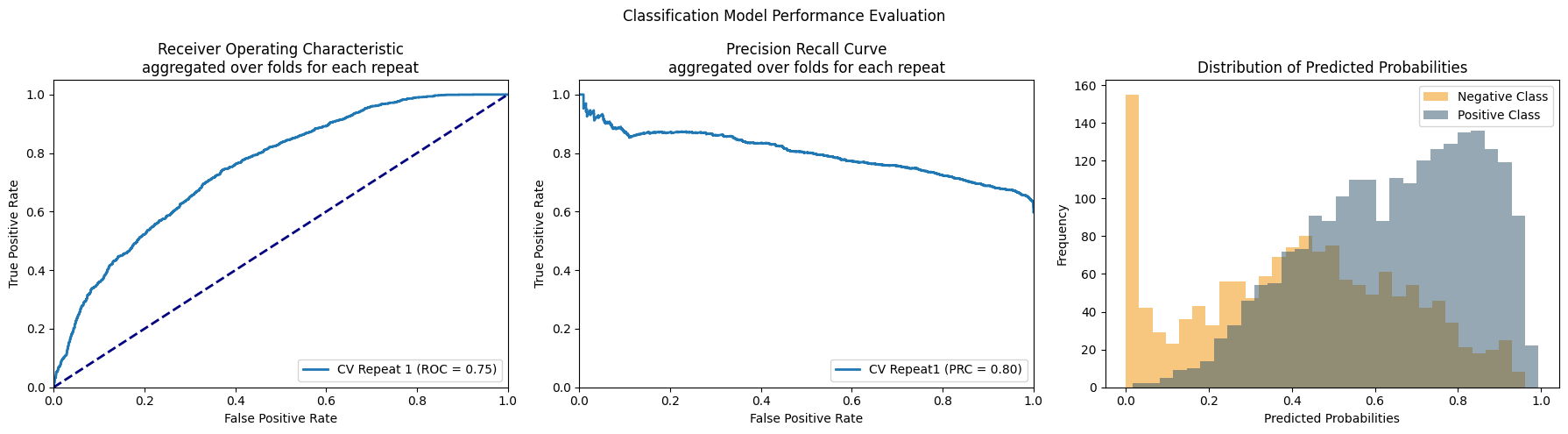
Step 3: Run CellPhenoX - train the classification model and calculate the CellPhenoX Interpretable Score
We start by instantiating the CellPhenoX object with CellPhenoX, specifying the following attributes:
outer_num_splits- the number of cross validation folds.inner_num_splits- the number of cross validation folds for the hyperparameter grid search.CV_repeats- the number of cross validation repeats to perform. This ensures that the SHAP values calculated are robust to the randomization of the folds; the final SHAP values for each cell for each feature will be the average across CV repeats.
other CellPhenoX object attributes
The function for running this step is model_training_shap_val. You can pass the path to a specific output path for the produced plots.
[11]:
# create CellPhenoX object
cellpx_obj = CellPhenoX(X, y, CV_repeats=1, outer_num_splits=3, inner_num_splits=2)
# and then train the classification model
cellpx_obj.model_training_shap_val(outpath = output_path)
entering CV loop

------------ CV Repeat number: 1

------ Fold Number: 1
--- Accuracy:  0.7023519870235199
1
--- Validation Accuracy:  0.8275862068965517  - Validation AUROC:  0.8185670261941448  - Val AUPRC:  0.9549581934555448

------ Fold Number: 2
--- Accuracy:  0.7055961070559611
2
--- Validation Accuracy:  0.9006085192697769  - Validation AUROC:  0.892869371682931  - Val AUPRC:  0.9770399352399095

------ Fold Number: 3
--- Accuracy:  0.6801948051948052
3
--- Validation Accuracy:  0.8765182186234818  - Validation AUROC:  0.8679925048973682  - Val AUPRC:  0.9707836787744281
Average AUROC: 0.8598096342581479 | Average AUPRC: 0.9675939358232942
best model precision-recall score = 0.9770
/Users/zhanglab_mac2/Library/CloudStorage/OneDrive-TheUniversityofColoradoDenver/Zhang_Lab/Research/shap/.conda/lib/python3.11/site-packages/shap/plots/_beeswarm.py:699: UserWarning: No data for colormapping provided via 'c'. Parameters 'vmin', 'vmax' will be ignored
The .shap_df attribute will hold the SHAP values for the individual features in the model (these columns will have the names of the features and “_shap”). The interpretable_score column holds the CellPhenoX Interpretable Score.
[12]:
cellpx_obj.shap_df
[12]:
| 0_shap | 1_shap | 2_shap | 3_shap | interpretable_score | |
|---|---|---|---|---|---|
| cell | |||||
| N7.LPA.ATGTTCACATCGAC | 0.019978 | -0.007582 | 0.129763 | 0.017164 | 0.159322 |
| N7.LPA.CATTAGCTGAGACG | 0.018379 | 0.019989 | 0.234010 | 0.130304 | 0.402682 |
| N7.LPA.AAGGCTTGTGTAGC | 0.052278 | 0.037604 | 0.184861 | -0.004939 | 0.269803 |
| N7.LPA.TATCAAGATGTGAC | 0.013674 | 0.056203 | 0.068779 | -0.102463 | 0.036193 |
| N7.LPA.GAGTGGGAATGTGC | -0.017015 | 0.016166 | -0.011645 | -0.110724 | -0.123219 |
| ... | ... | ... | ... | ... | ... |
| N110.LPB.CCAGCGATCCTCCTAG | -0.025661 | -0.084043 | -0.027967 | 0.075934 | -0.061737 |
| N110.LPB.CGAATGTAGACTAGGC | 0.047468 | 0.004443 | 0.219336 | -0.048841 | 0.222407 |
| N110.LPB.TCAACGACAATCCAAC | 0.076038 | 0.083048 | 0.001184 | 0.036729 | 0.196999 |
| N110.LPB.CTGATAGAGCATGGCA | -0.014526 | 0.030951 | -0.008796 | 0.198806 | 0.206434 |
| N110.LPB.CTTCTCTCATCGGTTA | 0.012489 | 0.024917 | 0.012230 | 0.262411 | 0.312047 |
3698 rows × 5 columns
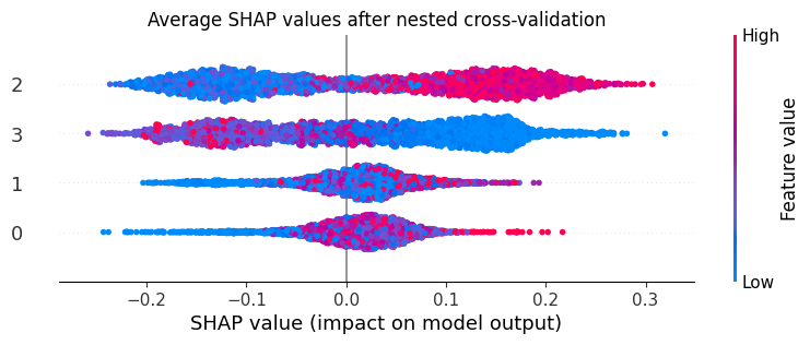
Step 4: Visualization - generate manuscript plots
SHAP Summary plot
(inlcude option to keep the covariates in the plot)
Boxplots with CellPhenoX Interpretable Score on the y-axis
CellPhenoX Interpretable Score on the UMAP & Celltype labeled UMAP
We include the code for correlating the Interpretable Score with the gene expression in (this notebook). In general, the steps are as follows….
[13]:
marker_discovery(cellpx_obj.shap_df, expression_mat)
fitting model
/Users/zhanglab_mac2/Library/CloudStorage/OneDrive-TheUniversityofColoradoDenver/Zhang_Lab/Research/shap/.conda/lib/python3.11/site-packages/statsmodels/regression/linear_model.py:1794: RuntimeWarning: divide by zero encountered in divide
/Users/zhanglab_mac2/Library/CloudStorage/OneDrive-TheUniversityofColoradoDenver/Zhang_Lab/Research/shap/.conda/lib/python3.11/site-packages/statsmodels/regression/linear_model.py:1794: RuntimeWarning: invalid value encountered in scalar multiply
/Users/zhanglab_mac2/Library/CloudStorage/OneDrive-TheUniversityofColoradoDenver/Zhang_Lab/Research/shap/.conda/lib/python3.11/site-packages/statsmodels/regression/linear_model.py:1716: RuntimeWarning: divide by zero encountered in scalar divide
results sorted by p vlaue:
              Beta  P_Value  Adjusted_P_Value      gene
const     0.007220      NaN               NaN     const
ADAMDEC1  0.009512      NaN               NaN  ADAMDEC1
ACTA2    -0.004977      NaN               NaN     ACTA2
TAGLN     0.002539      NaN               NaN     TAGLN
CCL11    -0.005101      NaN               NaN     CCL11
Significant Markers
Empty DataFrame
Columns: [Beta, P_Value, Adjusted_P_Value, gene]
Index: []